Introduction to academiadates

I’ve created the academiadates package to extend support of the tidyverts ecosystem handling a specific pattern of dates. The pattern of dates is academic terms, hence the name. Most institutions that I’m aware of use three terms per calendar year: spring, summer, and fall.

The tsibble package provides a new data frame class, the tsibble, and a handful of classes for various time intervals. Those are covered on the {tsibble} home page. This package provides a new class, yeartrimester, which is suited to handle three terms in a similar way as yearquarter.

Creation

library(academiadates)
library(tsibble)
library(tsibbledata) # an example dataset
library(dplyr)

We have the following dataset from tsibbledata which is monthly data with counts of Australian livestock used for food.

aus_livestock
#> # A tsibble: 29,364 x 4 [1M]
#> # Key:       Animal, State [54]
#>       Month Animal                     State                        Count
#>       <mth> <fct>                      <fct>                        <dbl>
#>  1 1976 Jul Bulls, bullocks and steers Australian Capital Territory  2300
#>  2 1976 Aug Bulls, bullocks and steers Australian Capital Territory  2100
#>  3 1976 Sep Bulls, bullocks and steers Australian Capital Territory  2100
#>  4 1976 Oct Bulls, bullocks and steers Australian Capital Territory  1900
#>  5 1976 Nov Bulls, bullocks and steers Australian Capital Territory  2100
#>  6 1976 Dec Bulls, bullocks and steers Australian Capital Territory  1800
#>  7 1977 Jan Bulls, bullocks and steers Australian Capital Territory  1800
#>  8 1977 Feb Bulls, bullocks and steers Australian Capital Territory  1900
#>  9 1977 Mar Bulls, bullocks and steers Australian Capital Territory  2700
#> 10 1977 Apr Bulls, bullocks and steers Australian Capital Territory  2300
#> # ℹ 29,354 more rows

Notice how the first month is July. We can set the fiscal or academic year to start the seventh month for the sake of having a whole first year.

As an example we can aggregate this to quarters and trimesters. We have to convert to a regular tibble to make regrouping the data under the new time index easier.

# quarters
aus_q <- aus_livestock |> 
    as_tibble() |> 
    mutate(Quarter = yearquarter(Month, fiscal_start = 7)) |> 
    summarize(
        Count = sum(Count),
        .by   = c(Quarter, Animal, State)
    ) |> 
    as_tsibble(index = Quarter, key = c(Animal, State))

# trimesters
aus_t <- aus_livestock |> 
    as_tibble() |>
    mutate(Trimester = yeartrimester(Month, academic_start = 7)) |>
    summarize(
        Count = sum(Count),
        .by   = c(Trimester, Animal, State)
    ) |> 
    as_tsibble(index = Trimester, key = c(Animal, State))

aus_q
#> # A tsibble: 9,788 x 4 [1Q]
#> # Key:       Animal, State [54]
#>    Quarter Animal                     State                        Count
#>      <qtr> <fct>                      <fct>                        <dbl>
#>  1 1977 Q1 Bulls, bullocks and steers Australian Capital Territory  6500
#>  2 1977 Q2 Bulls, bullocks and steers Australian Capital Territory  5800
#>  3 1977 Q3 Bulls, bullocks and steers Australian Capital Territory  6400
#>  4 1977 Q4 Bulls, bullocks and steers Australian Capital Territory  7700
#>  5 1978 Q1 Bulls, bullocks and steers Australian Capital Territory  7000
#>  6 1978 Q2 Bulls, bullocks and steers Australian Capital Territory  6900
#>  7 1978 Q3 Bulls, bullocks and steers Australian Capital Territory  7800
#>  8 1978 Q4 Bulls, bullocks and steers Australian Capital Territory  8500
#>  9 1979 Q1 Bulls, bullocks and steers Australian Capital Territory  7900
#> 10 1979 Q2 Bulls, bullocks and steers Australian Capital Territory  7900
#> # ℹ 9,778 more rows

aus_t
#> # A tsibble: 7,368 x 4 [1T]
#> # Key:       Animal, State [54]
#>    Trimester Animal                     State                        Count
#>        <tri> <fct>                      <fct>                        <dbl>
#>  1   1977 T1 Bulls, bullocks and steers Australian Capital Territory  8400
#>  2   1977 T2 Bulls, bullocks and steers Australian Capital Territory  7600
#>  3   1977 T3 Bulls, bullocks and steers Australian Capital Territory 10400
#>  4   1978 T1 Bulls, bullocks and steers Australian Capital Territory  9300
#>  5   1978 T2 Bulls, bullocks and steers Australian Capital Territory  9600
#>  6   1978 T3 Bulls, bullocks and steers Australian Capital Territory 11300
#>  7   1979 T1 Bulls, bullocks and steers Australian Capital Territory 10700
#>  8   1979 T2 Bulls, bullocks and steers Australian Capital Territory 10100
#>  9   1979 T3 Bulls, bullocks and steers Australian Capital Territory  8000
#> 10   1980 T1 Bulls, bullocks and steers Australian Capital Territory  7300
#> # ℹ 7,358 more rows

If your date is in a format like Fall 2025, you can covert it to yeartrimester using seasonal_trimester(). This is set up to work for fall, spring, and summer terms.

Plotting

The built-in plotting functionality is limited. The plotting functionality for the tidyverts ecosystem is partly from the feasts package: Graphics. Some of those functions depend on the class of the index. This means that, without porting those functions to accommodate the yeartrimester class, a portion of the functionality will not work.

(I hope to do that in the future, but the functionality can be recreated manually for the time being.)

library(ggplot2)

aus_t |> 
    filter(
        Animal == "Bulls, bullocks and steers",
        Trimester >= yeartrimester('2012 T1', academic_start = 7)
    ) |> 
    ggplot(
        aes(
            x = Trimester,
            y = Count,
            color = State
        )
    ) +
    geom_line()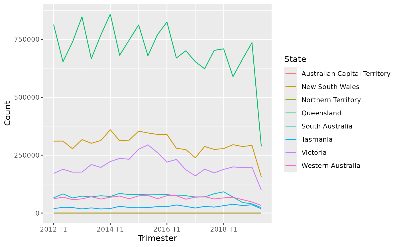

There is a bug in tsibble when using yearquarter with a fiscal_start. yearquarter_trans does not account for that offset, so the fiscal_start is dropped through transforming to a date and then inverting the transform.

I’ve worked around this by adding in the additional months to it when transforming to a date. The re-transformed yeartrimester does not have an offset, but the offset is built-in.

Steven Carter

Creation

Plotting